Import 3d buildings in Rhino

A step-by-step workflow for pulling building footprints with heights from the EUBUCCO database, trimming them to a study area in QGIS, and extruding them into a 3D massing model in Rhino via Grasshopper + Heron.

The method works for any European location covered by EUBUCCO.

---

Overview

The pipeline has two halves:

1. QGIS — download data, define your study area, trim the buildings to it, export.
2. Rhino + Grasshopper — import the footprints, extrude each one by its height attribute, cap into solids.

The single most important thing to keep consistent throughout is the coordinate reference system (CRS / EPSG code). Get that right and everything lines up; get it wrong and your model ends up tiny, distorted, or on the other side of the planet.

---

Part 1 — QGIS

Step 1.1 — Download the EUBUCCO data

1. Go to the EUBUCCO v0.2 files page: https://eubucco.com/files/v0.2
2. Find the region that contains your site. EUBUCCO v0.2 is split by NUTS2 region.
3. Download the GPKG file for that region. The GeoPackage bundles the building footprints and their attributes (height, floors, source, etc.) in a single file.

Step 1.2 — Install the Site Extent Tool plugin

The Site Extent Tool is a small plugin that draws a square or circle of a chosen size, centered on a point you click. It is how you will define your study area.

1. Download the plugin zip: site_extent_tool.zip
2. In QGIS, open Plugins → Manage and Install Plugins → Install from ZIP.
3. Browse to site_extent_tool.zip and click Install Plugin.
4. Accept the security prompt (this appears for any plugin not installed from the official QGIS repository — it is expected).
5. A new button appears on the toolbar, and an entry under Vector → Site Extent Tool.

Step 1.3 — Open the GPKG in QGIS

1. Open QGIS with a fresh project.
2. Drag the downloaded .gpkg file straight onto the map canvas. (Or: Layer → Add Layer → Add Vector Layer, browse to the file, Add.)
3. If a Select Items to Add dialog appears (a GeoPackage can hold several tables), tick the buildings layer and click Add Layers.

The footprints cover the whole NUTS2 region, so it will look like one big blob until you zoom in.

Step 1.4 — Set the project CRS

This step must happen before you draw your study area, because the Site Extent Tool measures size in the project's units.

1. Click the CRS button in the bottom-right corner of the QGIS window (usually something like EPSG:#### is written there).
2. Set the project CRS to your chosen metric system — EPSG:2154 for France.
3. Layers reproject on the fly, so the EUBUCCO data (stored in EPSG:3035) still displays in the right place.

Step 1.5 — Zoom to your site

1. If you have another layer for your specific site (your own building, an OSM export), add it and right-click → Zoom to Layer.
2. Otherwise, use the QGIS search/coordinate box or pan manually to find your site within the region.

Step 1.6 — Draw the study area (square or circle)

1. Click the Site Extent Tool button on the toolbar, or Vector → Site Extent Tool.
2. In the dialog:
   • Choose Shape: Square or Circle.
   • Enter the size in meters. For a square this is the side length; for a circle it is the diameter. A value of 1000 gives a 1 km square (500 m in each direction) or a 1 km-diameter circle.
3. Click Pick centre on map.
4. Click the point on the map where you want the centre of your study area.
5. A new memory layer appears — e.g. site_square_1000m — centred on your click.

Step 1.7 — Trim the buildings to the study area

Now clip the region-wide buildings down to just your study area.

1. Open Vector → Geoprocessing Tools → Clip.
2. Set:
   • Input layer = the EUBUCCO buildings layer.
   • Overlay layer = your site_square_1000m (or circle) layer.
3. Run. A new clipped layer contains only the buildings inside your study area.

Step 1.8 — Check the height attribute

Before exporting, confirm the heights are there.

1. Right-click the clipped layer → Open Attribute Table.
2. Find the height field (values in metres) and the source / provenance field.
3. Sort by height to see how many buildings have values versus empty / nan.

Step 1.9 — Export to Shapefile

Rhino and Heron read Shapefiles cleanly, so export the clipped layer as .shp.

1. Right-click the clipped layer → Export → Save Features As…
2. Set:
   • Format = ESRI Shapefile
   • CRS = EPSG:2154 (keep it consistent with your project)
   • File name = somewhere easy to find, e.g. buildings_site.shp
3. Click OK.

Part 2 — Rhino + Grasshopper

Step 2.1 — Install Heron

Heron is the Grasshopper plugin that reads GIS data (Shapefiles, GeoJSON) and handles reprojection.

1. In Rhino, run the PackageManager command (type it into the command line).
2. Search for Heron.
3. Click Install, then restart Rhino.

Step 2.2 — Set the file units to meters

Your data is in meters, so Rhino must be too.

1. Tools → Options → Units (or File → Properties → Units).
2. Set Model units to Meters.
3. Do this on a fresh file before importing, so nothing gets scaled unexpectedly.

Step 2.3 — Open Grasshopper and build the definition

Open Grasshopper (Grasshopper command) and build the following definition.

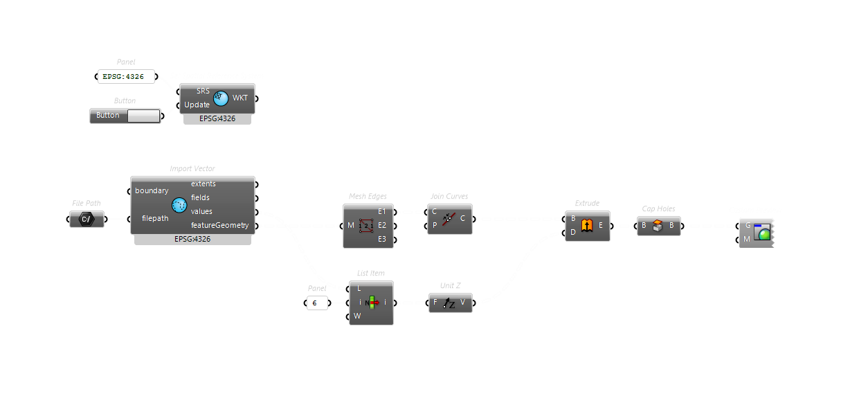
The definition does this, left to right:

1. File Path → points to your buildings_site.shp.
2. Set Spatial Reference System (SRS) → set to EPSG:2154 so Heron keeps the data in metres (matching your QGIS export). Feed this into Import Vector's SRS so it does not fall back to WGS84.
3. Import Vector → reads the Shapefile. Outputs:
   • featureGeometry — the footprints
   • fields — the list of attribute names
   • values — the attribute values, as a tree (one branch per building)
4. List Item on values, index 6 → pulls the height value for each building. (Index 6 matches the EUBUCCO field order: fid, id, region_id, city_id, type, subtype, height, …)
5. Clean the heights → replace empty / nan entries with a fallback (e.g. an Expression if(x > 0, x, 6)) so every building has a usable number.
6. Unit Z × height → builds a vertical extrusion vector per building.
7. Extrude (footprint curve + vector) → raises each footprint to its height.
8. Cap Holes → closes the open tops/bottoms into solid Breps.

Step 2.4 — Bake and move to the origin

1. When the solids look right, bake the geometry into Rhino.
2. The model will sit hundreds of kilometres from the origin, because EPSG:2154 coordinates are large. This causes display and precision issues.
3. Select all → Move → from a known reference point to 0,0,0.

---

CRS consistency checklist

The whole pipeline only works if the CRS is consistent. Tick these off:

Stage	What to check	Should be
EUBUCCO file	Native storage CRS	EPSG:3035 (handled by QGIS automatically)
QGIS project	Project CRS (bottom-right)	EPSG:2154
Site Extent Tool	Inherits project CRS	EPSG:2154
Shapefile export	Export CRS + .prj present	EPSG:2154
Heron Set SRS	Matches export	EPSG:2154
Rhino	Model units	Meters

---

Summary

1. Download the EUBUCCO GPKG for your NUTS2 region.
2. Install the Site Extent Tool plugin from ZIP.
3. Open the GPKG, set the project to a metric CRS, draw your square/circle, Clip the buildings to it.
4. Export the clipped layer as Shapefile in the same CRS.
5. In Rhino: install Heron, set units to Meters, build the Grasshopper definition to import → pull height → extrude → cap.
6. Bake and move to origin.
7. Keep the CRS consistent at every stage.

You now have a 3D massing model of your site, ready for environmental and design analysis.